One of the challenges to finding optimal solutions is the coupling of variables. If we could change one variable at a time, the search process would be so much easier. But in most problems the variables are strongly coupled, so the best value for one variable depends on the values of many other variables.
Often, we have no control over this variable coupling, since it is inherent in the physics model that defines our objectives and constraints. In these cases, we need a powerful optimization search strategy like SHERPA to figure out the complexities of the design landscape and to produce an optimized solution.
But in some cases we make this task harder than it needs to be because of how we represent the problem. That is, sometimes the way we define the problem creates unnecessary coupling or increases the complexity of existing coupling among variables. This makes the optimization search harder, and may decrease the chance of finding the optimal solution within our limited optimization search budget. The good news is that we can often alleviate this situation with a different representation.
Let’s consider an example. This example is simple on purpose, in order to illustrate the concept. You can apply these ideas to much more complicated situations with similar benefits.
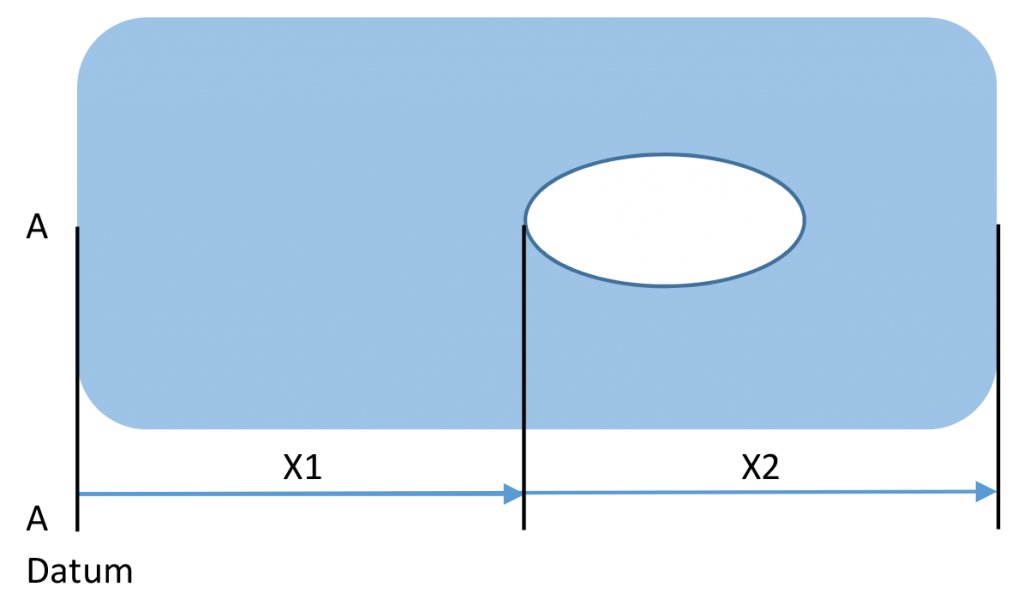
A common optimization scenario is the determination of optimal dimensions and feature locations to meet a specific performance goal. Suppose we wish to optimize a flat plate, and our performance goal depends strongly on the location of an elliptical hole and the length of the plate. We could represent these two variables as X1 and X2 in a parametric geometry model as shown in Figure 1 below. For now, let’s assume that the allowable ranges for X1 and X2 maintain the elliptical hole within the outer dimensions of the plate.

Figure 1. Parametric geometry model with two independent design variables X1 and X2. AA is a datum plane.
During the mathematical search for optimal values of X1 and X2, designs may be found that have a good value for the length of the plate, but the location of the hole is not yet ideal. Unfortunately, changing the location of the hole (X1) also changes the length of the plate (X1+X2), so our selection of design variables has introduced a strong coupling between hole location and plate length in our design landscape.
If the hole location and the plate length were already strongly coupled through the physics model that defines performance, then our representation of this problem might not make a large difference. However, if these two parameters were weakly coupled or not coupled at all in the physics model, then our representation in Figure 1 would increase the complexity of our problem, perhaps significantly.
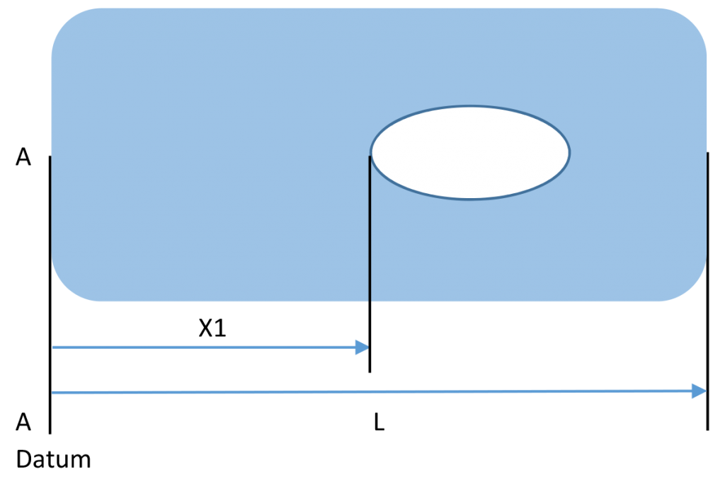
A better representation would be as shown below in Figure 2, where we use X1 and L as our variables. Since both X1 and L are measured from a fixed datum, they are geometrically independent. The only the coupling present now is due to the physics model of the performance function, which we cannot control.

Figure 2. Preferred parametric geometry model with two independent design variables X1 and L, both measured from a datum plane AA.
It is not always possible to know if our representations are ideal, so we are fortunate to have powerful optimization technology that can handle the complexity of our problems.
But we can often identify a less than ideal problem definition by simply thinking about (or visualizing, in the case of geometric variables) the effects that changing one variable will have on other variables in the problem. By spending some time to identify and reduce unintended coupling or other consequences in our problem representation, we may simplify the design landscape considerably.
We hope this tip helps you to find better designs, faster.