We often need for a design or a model to perform in a specified way. For example, the parameters in a nonlinear material model should be selected to best match the experimental stress-strain response. The geometrical parameters of a rubber bushing should be designed so that its force-deflection response matches the desired nonlinear stiffness behavior.
Optimization problems like these arise frequently. We refer to them as curve-fitting problems, because the goal is to minimize the difference between the specified target curve and the actual response curve
of our design or model.
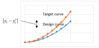
Figure 1. The difference between a target curve and a design curve is minimized in a curve fitting optimization problem.
When comparing two curves, it is necessary to develop a single, scalar measure of how well these two curves match one another. A common measure is the Root Mean Square Error (RMSE). For a simple function ![]() , the RMSE is calculated as follows:
, the RMSE is calculated as follows:
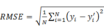
(Equation 1)
where: ![]() is the number of points
is the number of points ![]() at which the curves are compared,
at which the curves are compared, ![]() points on the actual (design) curve and
points on the actual (design) curve and ![]() are points on the target curve. A smaller value of RMSE indicates a better match between the curves.
are points on the target curve. A smaller value of RMSE indicates a better match between the curves.
HEEDS MDO has a built-in function to calculate the RMSE between two curves. So you only need to specify points on the target curve and define the two analysis model responses corresponding to the x and y values of points on the design curve. The objective in the optimization statement is then stated as:
Minimize: RMSE
If multiple curves need to be matched at the same time, then it is necessary to define a separate RMSE value for each curve. If there are three curves to be matched, for example, then the final objective
function can be written as the sum:
Minimize: w1*RMSE1 + w2*RMSE2 + w3*RMSE3
where wi are weighting factors that can be used to emphasize one or more RMSE values that are more important or more difficult to minimize. For example, if Curve 2 is the most important one to match accurately, then we could set: w1=1, w2=5, w3=1.
An example of a problem with multiple target curves is a strain rate sensitive material model, in which the material model must match the experimental stress-strain response for several strain rates.
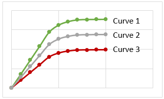
Figure 2. Multiple target curves that must be
matched by the same design or model.
Similarly, if a single curve has multiple parts, it is often advantageous to define a separate RMSE function for each part of the curve. If the curve has been divided into two parts, then the final objective function can be written as the sum:
Minimize: w1*RMSE1 + w2*RMSE2
For example, in a material that exhibits hysteresis the loading and unloading parts of the stress-strain curve are different. It would be difficult to use Equation (1) directly for this problem, but it is straightforward to split the curve into two parts, as shown in Figure 3.
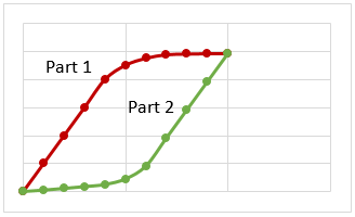
Figure 3. Multiple parts of a single target curve
that must be matched.
The most obvious examples of curve-fitting problems seem to be matching material models to experimental data. But there are numerous design studies where the goal is to match the response of a design to a preferred, or target curve. For example:
- Match the outlet velocity profile of a fluid in a tube to a desired outlet velocity distribution. If the outlet velocity profile is axisymmetric or varies in only one direction, then it can be solved directly as describe above. If the outlet velocity profile varies in two dimensions over the cross-section of the tube, then a script can be written to calculate the RMSE for a surface fit.
- Match the force-time history (the crash pulse) of an automotive crush tube to an ideal response curve.
- Match automotive camber, caster, and toe curves to desired curves for vehicle handling
- Tune a ride quality model to better match measured on-road vibration data
- Tune the boundary conditions of haemodynamic models to match measured upstream or downstream blood flow characteristics
And there are many others. As a small variant on the curve-fitting problem, sometimes the goal of an optimization study is to maintain the design response to be always above or below a specified target curve. These two cases are also easily defined directly in HEEDS.
Even though curve-fitting problems are relatively easy to define, they are often not easy to solve. In fact, some curve fitting problems are among the most challenging optimization search problems. For this reason, it is important to use a powerful optimization search technology that thoroughly explores the design space while refining the solution locally at the same time, like SHERPA does.
We hope this tip helps you to find better designs, faster.